


By Shimshon Bichler and Jonathan Nitzan
September 24, 2020
What do economists mean when they talk about “capital accumulation”? Surprisingly, the answer to this question is anything but clear, and it seems the most unclear in times of turmoil. Consider the “financial crisis” of the late 2000s. The very term already attests to the presumed nature and causes of the crisis, which most observers indeed believe originated in the financial sector and was amplified by pervasive financialization.
However, when theorists speak about a financial crisis, they don’t speak about it in isolation. They refer to finance not in and of itself, but in relation to the so-called real capital stock. The recent crisis, they argue, happened not because of finance as such, but due to a mismatch between financial and real capital. The world of finance, they complain, has deviated from and distorted the real world of accumulation.
According to the conventional script, this mismatch commonly appears as a “bubble”, a recurring disease that causes finance to inflate relative to reality. The bubble itself, much like cancer, develops stealthily. It is extremely hard to detect, and as long as it’s growing, nobody – save a few prophets of doom – seems able to see it. It is only after the market has crashed and the dust has settled that, suddenly, everybody knows it had been a bubble all along. Now, bubbles, like other deviations, distortions and mismatches, are born in sin. They begin with “the public” being too greedy and “policy makers” too lax; they continue with “irrational exuberance” that conjures up fictitious wealth out of thin air; and they end with a financial crisis, followed by recession, mounting losses and rising unemployment – a befitting punishment for those who believed they could trick Milton Friedman into giving them a free lunch.
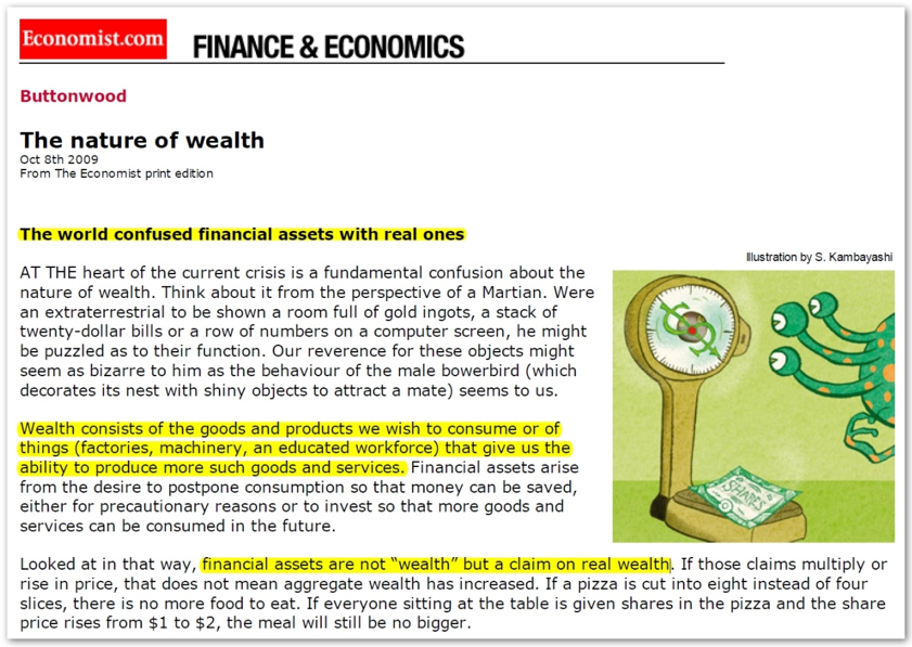
This “mismatch thesis” – the notion of a reality distorted by finance – is broadly accepted. In 2009, The Economist of London accused its readers of confusing “financial assets with real ones”, singling out their confusion as the root cause of the brewing crisis (Figure 1). Real assets, or wealth, the magazine explained, consist of “goods and products we wish to consume” or of “things that give us the ability to produce more of what we want to consume”. Financial assets, by contrast, are not wealth; they are simply “claims on real wealth”. To confuse the inflation of the latter for the expansion of the former is the surest recipe for disaster.
Figure 1: The classical dichotomy: real and financial
The division between real wealth and financial claims on real wealth is a fundamental premise of political economy. This premise is accepted not only by liberal theorists, analysts and policymakers, but also by Marxists of various persuasions. And as we shall show below, it is a premise built on very shaky foundations.[2]
When liberals and Marxists say that there is a mismatch between financial and real capital, they are essentially making, explicitly or implicitly, three related claims: (1) that these are indeed separate entities; (2) that these entities should correspond to each other; and (3) that, in the actual world, they often do not.
In what follows, we explain why these claims don’t hold water. To put it bluntly, neither liberals nor Marxists know how to compare real and financial capital, and the main reason is simple: they don’t know how to determine the magnitude of real capital to start with. The common, makeshift solution is to estimate this magnitude indirectly, by using the money price of capital goods – yet this doesn’t solve the problem either, since capital goods can have many prices and there is no way of knowing which of them, if any, is the “true” one. Last but not least, even if we turn a blind eye and allow for these logical impossibilities and empirical travesties to stand, the result is still highly embarrassing. As it turns out, financial accumulation not only deviates from and distorts real accumulation (or so we are told), it also follows an opposite trajectory. For more than two centuries, economists left and right have argued that capitalists – and therefore capitalism – thrive on “real investment” and the growth of “real capital”. But as we shall see, in reality, the best time for capitalists is when their “real accumulation” tanks! . . .
2. The duality of real and nominal
The basic dualities of subject and object, idea and thing, nomos and physis have preoccupied philosophers since antiquity. They have also provided an ideal leverage for organized religions and other dogmas specializing in salvation from alienation. And more recently, they have come to form the basic foundation of modern economics.
Get Evonomics in your inbox
Following the “classical dichotomy” proposed by the British philosopher David Hume, economists divide their economy into two parallel worlds: real and nominal. The more important of the two realms, by far, is the real economy. This is the domain of scarcity, the arena where demand and supply allocate limited resources among unlimited wants. It is where production and consumption take place, where sweat and tears are shed and desires fulfilled, where factors of production mix with technology, where capitalists invest for profit and workers labour for wages. It is where conflict meets cooperation, the anonymous forces of the market engage the visible hand of power, exploitation takes place and actual capital accumulates. It is the raison d’être of social reproduction, the locus of action, the means and end of economics. In short, it is the real thing.
The nominal economy merely reflects this reality. Unlike the real economy, with its productive efforts, tangible goods and useful services, the nominal sphere is entirely symbolic. Its various entities – fiat money and money prices, credit and debt, equities and securities – are all denominated in dollars and cents (or any other currency units). They are counted partly in minted coins and printed notes, but mostly in electronic bits and bytes. This is a parallel universe, a world of mirrors and echoes, a bare image of the real thing.
This real-nominal duality cuts through the whole of economics, including capital. For economists, capital comes in two varieties: real capital (wealth) and financial capital (capitalization). Real capital is made of “capital goods”. It comprises means of production, including plant and equipment, infrastructure, work in progress and, according to many, knowledge. Financial capital, or capitalization, represents a symbolic claim on this real capital. Its quantity measures the present value of the earnings that the underlying capital goods are expected to yield.
Both Marxists and neoclassicists accept the real/nominal bifurcation of the economy. They also accept that there are two types of capital – real and financial. And they also believe (in the Marxist case) and concede (in the neoclassical case) that, usually, there is a mismatch between them. The main difference between the two schools is the direction of the mismatch: Marxists begin with a mismatch that they argue must turn into a match, whereas neoclassicists begin with a match that, they reluctantly admit, often disintegrates into a mismatch. So let’s examine this difference a bit more closely, beginning with the Marxist view.[3]
2.1 The Marxist View
Marx wrote in the middle of the nineteenth century, roughly half a century before others started to theorize capitalization in earnest and a full century before it became the central ritual of modern capitalism. Yet he was prescient enough to understand the importance of this process and tried to sort out what it meant for his labour theory of value.
He started by stipulating two types of capital: actual and fictitious. Of these two, the key was actual capital – means of production and work in progress counted in labour time. This was “real” capital. Fictitious capital – or capitalization – was the magnitude of expected future income discounted to its present value. This later capital, counted in dollars and cents, was deemed fictitious for three basic reasons: (1) often there is no “principal” to call on (as in the case of government debt, where the creditor owns not actual capital, but merely a claim on government revenues); (2) capitalization is based on changing income expectations that may or may not materialize; and (3) even if the expected income is given, its capitalized value varies with the discount rate.
The existence of two types of capital created a dilemma for Marx. Theoretically, actual and fictitious capital are totally different creatures with totally different magnitudes. But the capitalist reality is denominated in prices, which means that, in practice, real and fictitious capital are deeply intertwined. This latter fusion, says Marx, leads to massive distortions, particularly during a boom, often to the point of making the entire process of accumulation “unintelligible”:
All connection with the actual process of self expansion of capital is thus lost to the last vestige, and the conception of capital as something which expands itself automatically is thereby strengthened. . . . The accumulation of the wealth of this class [the large moneyed capitalists] may proceed in a direction very different from actual accumulation. . . . Moreover, everything appears turned upside down here, since no real prices and their real basis appear in this paper world, but only bullion, metal coin, notes, bills of exchange, securities. Particularly in the centers, in which the whole money business of the country is crowded together, like London, this reversion becomes apparent; the entire process becomes unintelligible. (Marx, Karl. 1894. Capital. A Critique of Political Economy. Vol. 3: The Process of Capitalist Production as a Whole. Edited by Friedrich Engels. New York: International Publishers, pp. 549, 561, 576, emphasis added)
Marx’s followers solved this problem by assuming that, over the long run, the labour theory of value prevails (with prices proportionate to labour values) and therefore that, at some point, there must be a “financial” crisis to bring the price of fictitious capital back in line with the labour values of real capital:
In order for the price system to work, financial forces should cause fictitious capitals to move in directions that parallel changes in reproduction values. . . . By losing any relationship to the underlying system of values, strains eventually build up in the sphere of production until a crisis is required to bring the system back into a balance, whereby prices reflect the real cost of production. The fiction of fictitious value cannot be maintained indefinitely. At some unknown time in the future, prices will have to return to a rough conformity with values. . . . (Perelman, Michael. 1990. The Phenomenology of Constant Capital and Fictitious Capital. Review of Radical Political Economics, Vol. 22, Nos. 2-3, p. 83),
2.2 Fisher’s House of Mirrors
On the neoclassical side, the duality of real and financial capital was articulated a century ago by the American economist Irving Fisher. This was the beginning of a process that contemporary commentators refer to as financialization, and whose logical structure Fisher was one of the first theorists to systematize. Table 1 and the quote below it outline his framework:
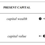
Table 1: Fisher’s House of Mirrors
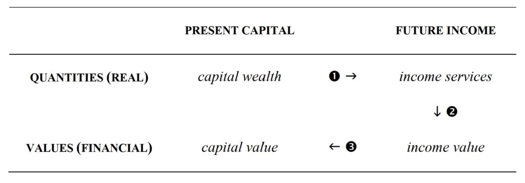
The statement that “capital produces income” is true only in the physical sense; it is not true in the value sense. That is to say, capital-value does not produce income-value. On the contrary, income-value produces capital-value. . . . [W]hen capital and income are measured in value, their causal connection is the reverse of that which holds true when they are measured in quantity. The orchard produces the apples; but the value of the apples produces the value of the orchard. . . . We see, then, that present capital-wealth produces future income-services, but future income-value produces present capital-value. (Irving Fisher, The Rate of Interest, 1907, NY: The Macmillan Company, pp. 13-14, original emphases)
In this quote, Fisher draws three basic links: (1) the stock of capital goods, which economists consider as wealth, generates future income services; (2) future income services generate corresponding future income values; and (3) future income values, capitalized in the here and now, give capital its financial value.
And so the ancient alienation of the thing from its idea is hereby resolved. The real capital on the asset side of the balance sheet is made equal to the financial capital on the liabilities side. The machines, structures, inventories and knowledge, taken as an aggregate magnitude, are equivalent to the sum total of the corporation’s equity and debt obligations. The nominal mirrors the real. The nomos and physis are finally made one and the same.
Now, admittedly, this is merely the ideal state, the ultimate equilibrium a free, rational economy is bound to achieve. Sadly, though – and as neoclassicists are at great pain to admit – we are not there yet. In practice, the here-and-now economy is constantly upset by shocks, imperfections and distortions that, regrettably, cause finance to deviate from its proper, real value and equilibrium to remain a distant goal.
3. The quantity of wealth
To sum up, then, Marxists and neoclassicists approach the real/nominal duality from opposite directions. In the Marxist case, the duality starts as a mismatch that is eventually forced into a match, whereas in the neoclassical case it begins as a match and gets distorted into a mismatch.
However, in both cases – and this is the key point – the benchmark is real or actual capital. This is the yardstick, the underlying quantity that finance supposedly matches or mismatches. At some point, be it at the beginning or the end of the process, the capitalized value of finance must equal the quantity of wealth over which it constitutes a claim. In other words, the entire exercise is built upon the material quantity of capital goods. The only problem is that nobody knows what this quantity is or how to measure it.
3.1 Utils and SNALT
During the 1960s, there was a very important controversy in economics, pitting heterodox professors from Cambridge University in England against some of their orthodox counterparts at MIT in Cambridge, Massachusetts. The U.K. economists claimed that orthodox economics was built on a basic fallacy: it treated capital as having a definite quantity while, in fact, such a quantity cannot be shown to exist. Capital, they demonstrated, can rarely if ever be measured in its own “natural” material units. And their U.S. counterparts eventually agreed. Reluctantly, they conceded that real capital was merely a “parable”. Like the ever elusive God, you can speak about it, but, generally, you cannot quantify it.
This Cambridge Controversy, as it later came to be known, has since been buried and forgotten. The textbooks don’t mention it, most professors haven’t heard about it and certainly don’t teach it, and the unexposed students remain blissfully ignorant of it.[4] The reason for the hush-hush is not hard to understand: to accept that real capital has no definite quantity is to terminate modern economics as we know it. In order to avoid this fate, the dismal scientists have taken the anti-scientific route of keeping their skeletons in the closet. They have ignored their own conclusions, gradually erased the very debate from their curricula and syllabi and fortified the walls surrounding their academic religion to ward off the infidels.
But the problem remains, and, given its devastating consequences, it is worth considering, if only briefly. The basic reason that real capital cannot be measured is aggregation. Considered as a productive economic entity, capital consists of qualitatively different objects: tractors are different from trucks, ships are different from airplanes and automobile factories are different from oil rigs. This heterogeneity explains why the heterodox Cambridge economists claimed that capital has no “natural unit”: there is no simply way to compare and add up its components, and that inability makes it difficult to decide “how big” or “how small”
it is.[5]
The common solution in such cases is reduction – i.e., going one step lower to devise a fundamental quantity common to all entities in question. Perhaps the first to employ this method was the Greek philosopher Thales, when he claimed that everything in the world was made of water. The same principle is used by physicists when they argue that every quantity in the universe can be expressed in terms of mass, distance, time, electrical charge or heat (so velocity = distance ÷ time; acceleration = rate of change of velocity; force = mass x acceleration, etc.).
Economists mimic this reductionism with their own fundamental quantities. For the neoclassicists, this quantity is the “util”, a measure denoting the hedonic pleasure generated by commodities.[6] Like any other commodity, every capital good has its own util-generating capacity, and if we add the individual util-generating capacities of different capital goods we get their aggregate measure as real capital. For instance, if one Toyota factory can produce 1 million utils and a BP oil rig can produce 2 million utils, their combined real capital is 3 million utils.
Classical Marxists do the very same thing with labour time. Every commodity, they say, can be measured by the socially necessary abstract labour time (SNALT) it takes to produce; and by adding up these times, we can calculate the aggregate real quantity of the capital in question. If a Toyota factory takes 100 million socially necessary abstract labour hours to produce and a BP oil rig takes 200 million hours, their total quantity is 300 million hours.
So far so good – but then here there arises a small but nasty problem: unlike the physicists, economists have never managed to actually measure their fundamental quantities. As far as we know, no liberal has ever observed a util, and no Marxist has ever identified a unit of SNALT. As they stand, these so-called “real quantities” are, in fact, entirely fictitious.
But the economists haven’t given up. Instead of measuring utils and SNALT directly, they go in reverse. God is revealed to us through his miracles, and the same, argue the economists, holds true for the fundamental quantities of economics: they reveal themselves to us through their prices. For a neoclassicist, a 1:2 price ratio between a Toyota factory and a BP oil rig means that the first entity has half the util quantity of the second, while for a classical Marxist this same price ratio is evidence that the SNALT quantity of the first entity is half that of the second.
This reverse solution is the bread and butter of all practical economics. It is a common procedure that all economists use and few, if any, question, let alone critique. It is employed by everyone, from official statisticians and government economists to Wall Street analysts and corporate strategists. And as our reader might by now suspect, it doesn’t work – at least not in the way it is supposed to.
3.2 Equilibrating the capital stock
To see why the reserve solution doesn’t work, consider Table 2 and Figure 2, which present the same information – first numerically and then graphically. The table and figure pertain to a hypothetical company, Energy User-Producer Inc., which owns two assets – automobile factories that use energy and oil rigs that produce it. To make the example simple, we assume that there is only one type of automobile factory and that all oil rigs are identical. In order to know “how much” capital of each type there is, all we need to do is count. Table 2 shows the number of each of these “real assets”: Column 1 shows the number of automobile factories as they change over time, and Column 2 shows the corresponding number of oil rigs. These same numbers are shown by the two series at the bottom of Figure 2. The next two columns in the table – 3 and 4 – display, for each year, the unit price of each type of asset, counted in millions of dollars.
Now, since automobile factories and oil rigs are different entities, they cannot be added in their own “natural” units. And since we don’t know their util or SNALT contents, we cannot add those numbers either. But we can follow the economic recipe of “revealed preferences” to backpedal from prices to utils or SNALT.
Get Evonomics in your inbox
Consider the neoclassical inversion.[7] In order to tease utils out of prices, all we need to do is identify a year of perfectly competitive equilibrium (PCE). So for argument’s sake, assume that this year happened to be 1970. This is a convenient assumption to make, because, in PCE, buyers and sellers are said to exchange commodities at prices proportionate to their util-denominated (marginal) preferences.[8] In our case here, the shaded/bold numbers in Table 2 show that, in 1970, an automobile factory cost $200 million and an oil rig cost $100 million (both hypothetical numbers). And since these are assumed to be PCE prices, their ratio presumably reveals that the util-generating capacity of an auto factory is twice that of an oil rig.
Now remember that in order to keep things simple, we also assumed that all automobile factories and oil rigs are the same, and that they remain unchanged over time. This assumption, together with our knowledge that 1970 was a year of PCE, allows us to easily calculate the overall quantity of capital owned by Energy User-Producer. All we need to do for every year is, first, multiply the number of automobile factories by 200 and the number of oil rigs by 100, and then sum up the two products. This calculation would then give us the util-generating capacity of the company, year in, year out, as shown in Column 5.
There is a nasty catch here, though.
Note that our calculations are premised on the assumption that PCE occurred in 1970 – but what if this assumption is wrong? What if PCE occurred not in 1970, but in 1974, when the price of oil was three times higher and inflation was running amok?
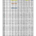
Table 2: The Many “Quantities” of Energy User-Producer Inc.
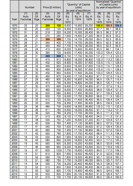
NOTES TO TABLE 2
The numbers of auto factories (Column 1) and oil rigs (Column 2) are hypothetical.
Column 5 = value of Column 3 in 1970 * Column 1 + value of Column 4 in 1970 * Column 2
Column 6 = value of Column 3 in 1974 * Column 1 + value of Column 4 in 1974 * Column 2
Column 7 = value of Column 3 in 1979 * Column 1 + value of Column 4 in 1979 * Column 2
Column 8 = Column 5 / value of Column 5 in 1970 * 100
Column 9 = Column 6 / value of Column 6 in 1970 * 100
Column 10 = Column 7 / value of Column 7 in 1970 * 100
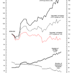
Figure 2: The Many “Quantities” of Energy User-Producer Inc.
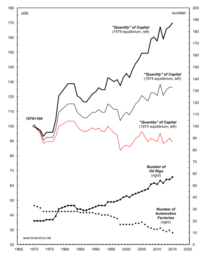
NOTE: The number of auto factories and oil rigs is hypothetical. The annual “quantity” of capital (in utils) is computed first by multiplying the number of auto factories and oil rigs by their respective equilibrium price; and second by adding the two products. The “quantity” of capital with a 1970 equilibrium assumes that the “util-generating capacities” of an auto factory and an oil rig have a ratio of 2:1 (based on respective prices of $200 mn and $100 mn); the “quantity” of capital with a 1974 equilibrium assumes that the ratio is 1:1 (based on respective prices of $300 mn and $300 mn); and the “quantity” of capital with a 1979 equilibrium assumes that the ratio is 1:2 (based on respective prices of $400 mn and $800 mn). For presentation purposes, all three quantity-of-capital series are normalized with the year 1970=100.
According to Table 2, in 1974 the price of automobile factories was $300 million apiece – 50 per cent higher than in 1970 – and the price of oil rigs was 200 per cent higher, at $300 million. Now, if we take these as our PCE prices and therefore as revealing the true util-generating capacity of the underlying assets, the quantity of capital would be very different than in the first scenario. Unlike before, the price ratio now is not 2:1, but 1:1, and that difference changes everything. The new results are shown in Column 6.
And the same question can be raised again: what if PCE occurred not in 1974, but in 1979, when inflation accelerated further and the price of oil rigs shot through the roof? According to Table 2, the price ratio now is 1:2, and that change, documented in Column 7, makes the quantities of capital different than in both previous scenarios.
In order to better compare the evolution of the capital stock under our three PCE settings, it is convenient to normalize Columns 5-7, as we do in Columns 8-10. For each of the Columns 5-7, we divide the quantity of capital by its value in 1970 and multiply the result by 100. This computation recalibrates the three series, bringing them all to a single common denominator, so that their respective values in 1970=100. Note that, because each observation in this transformation is divided and multiplied by the same numbers, the relative temporal changes of Columns 8-10 (although not the absolute numbers) are identical to those of Columns 5‑7, respectively.
The top part of Figure 2 shows the three normalized quantities of capital (Columns 8-10), each corresponding to a different PCE year. And as you can see, the trajectories of the series differ markedly from each other: if PCE occurred in 1970, the quantity of capital is shown to have declined by about 10 per cent over the entire period; if PCE occurred in 1974, though, the quantity of capital is shown to have increased by over 20 per cent; and if PCE occurred in 1979, the quantity of capital is seen to have risen by nearly 90 per cent.
3.3 So what is there to mismatch
Now, these are only three examples, and as our reader by now can imagine, we can give many others – in fact, as many as we wish – each based on a different PCE point and each yielding a different quantitative series. The crucial point here is that these different series all pertain to the same capital stock, so obviously only one of them, if any, can be “correct” – but which one is it?
Sadly, nobody knows.
As far as we can tell, nobody – not even top-of-the-line winners of the Nobel Memorial Prize in Economic Sciences – can identify PCE when they see it (assuming this is a meaningful social state to start with). And as long as PCE remains invisible, there is no way to decide which series, if any, shows the “true” magnitude of capital.
Similar problems haunt the Marxists. Given that SNALT is not directly observable, let alone measurable, Marxists, just like neoclassicists, are often forced to go in reverse. They deduce the labour-time magnitude of capital from the (PCE?) market prices of capital goods – or worse still, simply use the neoclassical, util-based measures provided by the national accounts.[9]
And so we’ve come full circle. The mismatch thesis claims that the quantity of financial capital deviates from and distorts the quantity of real capital. But as it turns out, the quantity of real capital – the thing that finance supposedly mismatches and distorts in the first place – is in fact totally nominal. Moreover, since this nominal quantity can be anything and everything (depending on our arbitrary choice of PCE), the economists are left with no unique (money) measure of real capital, let alone one they can all agree on. Caught in Plato’s cave, they try to glean reality from its reflection in their self-made mirror – only to discover that this mirror projects not one but an infinite number of images and that they have no idea how to choose between them. They end up with no real benchmark to match and therefore nothing to mismatch.
3.4 Flowing with the delusional crowd
In every other science, this inability to measure the key category of the theory would be devastating (think of measuring Newton’s gravitation without mass or distance). But not in the science of economics.[10]
Here, everything continues to flow smoothly. The national statistical services instruct their statisticians to come up with “real” numbers for the capital stock (as well as for every other economic entity). In order to comply, the statisticians have to identify instances of PCE; but since they too are clueless about the subject, they pretend. They designate an arbitrary year as their PCE, go through the hoops of Table 2, and churn out the required numbers. And although these official numbers are entirely fictitious, the economists, neoclassical as well as heterodox, don’t seem to care. They use them, usually without a second thought, as if they were the real thing.
So let’s not spoil the parade and, for the moment, continue to flow with the delusional crowd. For the sake of argument, let’s assume, along with the average economist, that, at any point in time, the dollar value of capital goods – or wealth, as Irving Fisher called them – is proportionate to the their real quantity, and then use this (pseudo) real measure as our basic benchmark.
With this assumption, we can now run a pragmatic test: we can take the financial magnitude of any capital (market capitalization) and compare it to its (fabricated) “real” benchmark (the aggregate money price of the underlying capital goods). According to Fisher’s neoclassical scriptures summarized in Table 1 – and assuming we are using the true PCE benchmark – the two quantities must equal. If they differ, reality must have been “distorted”.
4. Microsoft versus General Motors
The remainder of the paper draws its empirical illustrations from the United States. This focus, dictated largely by data availability, is of course limiting. But given that the U.S. was the leading engine of capitalism throughout much of the twentieth century and remains pivotal to contemporary global accumulation, its experience can still tell us plenty.
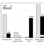
Figure 3 illustrates a simple case of “reality distorted by finance”. The chart, focusing on the year 2005, compares the so-called real and financial sides of two leading U.S. firms – Microsoft and General Motors. Seen from the real side, General Motors is a giant and Microsoft is a dwarf. In 2005, General Motors had 335,000 workers – 5.5 times more than Microsoft – and it had plant and equipment with a book value of 78 billion dollars – 33 times greater than Microsoft’s.
Figure 3: General Motors versus Microsoft, 2005
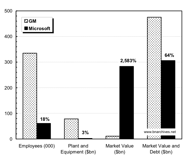
NOTE: The per cent figures indicate, for any given measure, the size of Microsoft relative to GM.
SOURCE: Compustat through WRDS (series codes: data29 for employees; data8 for net plant and equipment; data24 for price; data54 for common shares outstanding; data 181 for total liabilities).
But when we examine the two companies through the financial lens of capitalization, the pecking order is reversed: Microsoft becomes the giant and General Motors the dwarf. In 2005, Microsoft had a market capitalization nearly 26 times that of General Motors. Indeed, even if we take the sum of debt and market value, General Motors is still only 55 per cent bigger than Microsoft – a far cry from its relatively huge workforce and massive “quantity” of plant and equipment.
So, obviously, there must be some “distortion” here – for otherwise, how could a dwarf be a giant and a giant a dwarf?
Most economists, though, would shrug off the question. The problem, they would say, is that the chart shows only part of the picture. It measures real capital by looking at plant and equipment and the number of employees – yet neither of these magnitudes captures the importance of “technology”. This is a crucial omission, they would continue, for, as we all know, Microsoft is a high-tech company and therefore possesses much more technology than General Motors. And since technical knowhow affects market capitalization but rarely if ever gets counted as “plant and equipment” and has no bearing on the size of the companies’ workforce, our comparison is inherently lopsided. It demonstrates not a distortion but a simple mismeasurement.
And perhaps there is a mismeasurement here – but then, how can we be sure? Note that economists know the “magnitude” of technology here not by observing it directly (which nobody really can), but only indirectly, through its reflection in the mirror: they deduce it as the residual between market capitalization and the dollar value of plant and equipment.
Most economists encounter the technological “residual” in their study of production functions. These functions are intended to explain the level of output by the level of productive inputs – and are notoriously bad at doing so. Usually, they leave out a large unexplained variation in output – the infamous “residual” – whose existence the economists customarily blame on their inability to quantify “knowledge” (calling it a “measure of our ignorance”).
This inability has devastating consequences. To illustrate, consider two hypothetical production functions, with physical inputs augmented by technology: (1) Q = 2N + 3L + 5K + T and (2) Q = 4N + 2L + 10K + T, where Q denotes output, N labour, L land, K capital, and T technology. Now, suppose Q is 100, N is 10, L is 5 and K is 4. The implication is that T must be 45 in function (1) and 10 in function (2). Yet, since technology cannot be measured, we can’t know which production function is correct, so both – and, by extension, any technology-augmented function – can claim incontrovertible validity. But then, if production cannot be objectively described, what is left of the supply function, equilibrium and the entire edifice called economics?
The production-function residual is related to but different from the residual between capitalization and the real capital stock: the former supposedly measures the contribution of technology to output, whereas the latter presumably quantifies the actual magnitude of technology. However, both residuals share the property of being conveniently invisible and therefore irrefutable.
Now, what if the mirror of capitalization lies and the “residual” gives us a false reading? For example, what if it were in fact General Motors that possessed the “bigger” technology and the asset market simply “mispriced” the two stocks to erroneously suggest the opposite? And then there is the possibility – which we have graciously assumed way, though only as a freebie – that 2005 was a not a year of PCE, and therefore that our (nominal) measures of the real capital stock of the two companies are in fact distorted to start with. How do we know that the know-all market didn’t misprice these assets as well? And if there is no way of knowing, how can we say anything meaningful, let alone definitive, on the presumed “size” of technology?
5. Tobin’s Q: Adding Intangibles
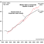
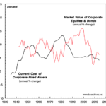
The same question, though on a much grander scale, arises from Figure 4. Whereas our comparison of Microsoft and General Motors is restricted to two firms at a point in time, in Figure 4 we look at all U.S. corporations from the 1930s to the present. The chart shows two series. The thick line is our (pseudo) real benchmark. It shows the current, or replacement, cost of corporate fixed assets (i.e., what they would cost to produce, every year, at prevailing rather than historical prices). The thin line is the corresponding magnitude of finance. It measures the total capitalization of corporate equities and bonds, an aggregate that constitutes a claim on and presumably mirrors the underlying sum total of real assets.
Figure 4: The “Quantity” of U.S. Capital
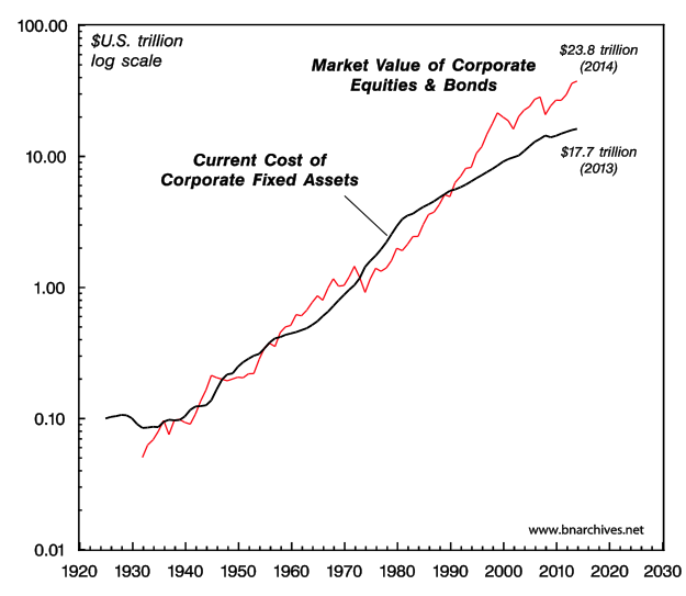
NOTE: The market value of equities and bonds is net of foreign holdings by U.S. residents.
SOURCE: U.S. Bureau of Economic Analysis through Global Insight (series codes: FAPNREZ for current cost of corporate fixed assets). The market value of corporate equities & bonds splices series from the following two sources. 1932-1951: Global Financial Data (market value of corporate stocks and market value of bonds on the NYSE). 1952-2014: Federal Reserve Board through Global Insight (series codes: FL893064105 for market value of corporate equities; FL263164103 for market value of foreign equities held by U.S. residents, including ADRs; FL893163005 for market value of corporate and foreign bonds; FL263063005 for market value of foreign bonds held by U.S. residents).
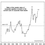
Note that we plot the two series against a log scale, so the discrepancies between them, although they look small on the graph, could be very large. These discrepancies are calibrated in Figure 5. The chart shows the Tobin’s Q index, named after the late economist James Tobin. For our purpose here, Tobin’s Q offers a sweeping measure of the financial-real mismatch. It computes, for every year, the ratio between the market value of corporations in the numerator and the replacement cost of their plant and equipment in the denominator. If finance matches reality, the two magnitudes are the same and Tobin’s Q will equal 1. If there is a mismatch, Tobin’s Q will exceed or fall short of 1.
Figure 5 has two notable features. First, it shows that the historical mean value of Tobin’s Q isn’t 1, but slightly above 1.2. Second, it demonstrates marked variations in Q, ranging from a low of 0.6 to a high of 2.5. These variations are not random, but rather cyclical and persistent. Let’s examine these two features more closely.
Figure 5: Tobin’s Q in the United States
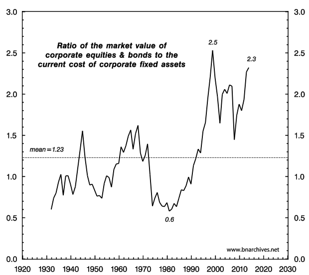
NOTE: The market value of equities and bonds is net of foreign holdings by U.S. residents. The last data point is for 2014 (based on the measured value of corporate equities and bonds and the estimated current cost of corporate fixed assets).
SOURCE: See Figure 4.
First, why is the historical average of Tobin’s Q greater than 1? The conventional answer, just like in the Microsoft-General Motors case, is mismeasurement. When physicists were unable to square their computations regarding the structure and expansion of the universe, they didn’t rush to change their theory; instead, they solved the problem, at least provisionally, by hypothesizing the existence of invisible “dark” matter whose assumed mass, when added to the mass of observed matter, would make their calculations consistent. Economists do the very same thing with the real-financial mismatch. The reason that capitalization tends to be larger than “real capital”, they say, is that fixed assets are only part of the picture. The other part is made of equally productive intangible assets. Unfortunately, most of these intangibles, like the physicists’ dark matter, are invisible. And it is this invisibility that explains why finance often mismatches reality and why Tobin’s Q averages more than 1.
Intangibles, many economists argue, have become more important since the 1980s’ onset of the “information revolution” and “knowledge economy” – exactly when Tobin’s Q started to soar. According to this view, corporations have accumulated more and more invisible assets in the form of improved technology, better organization, high-tech, synergy and other such knowledge-related blessings. These intangibles have in turn augmented the quantity of capital, and have therefore led to larger capitalization. Accountants, though, remain conservative, so most intangibles don’t get recorded as fixed assets on the balance sheet. And since the capitalized numerator of Tobin’s Q takes account of these intangibles while the fixed-asset denominator usually does not, we end up with a growing mismatch. By the mid-2000s, some guestimates suggested that intangibles have come to account for 80 per cent of all corporate assets – up from less than 20 per cent 30 years earlier.
Although popular, these claims are highly dubious. Just like in the Microsoft-General Motors case, here, too, intangible capital is computed as a residual, deduced by subtracting from market capitalization the value of fixed assets. Now if we accept this method – as most economists do – we must also accept that intangible capital is a highly flexible creature, capable of expanding rapidly (as it did during the 1980s and 1990s, when Tobin’s Q rose on a soaring market) as well as contracting rapidly (as it did during the major bear market of the 2000s, when Tobin’s Q tanked). But does this flexibility make any sense?
Given that technical knowhow tends to change very gradually and rarely contracts, how could its “magnitude” jump several-fold in a short decade, only to drop precipitately in the next? And that’s not all. To accept the residual method here is to concede that intangible capital can become negative – for otherwise, how could we account for Tobin’s Q falling below 1?
6. Boom and bust: irrationality
So what do the economists do to bypass these implausibilities? They add irrationality. The textbooks portray economic agents as rational and markets as efficient – but when pressed to the wall, even the fundamentalists admit that reality is rarely that pristine. In practice, economic agents are plagued by emotions, often misinformed and occasionally delusional. Moreover, and regrettably, the “market”, which the textbooks like to describe as perfect, is heavily contaminated and distorted by public officials and policymakers, oligopolies and insiders, labour unions and NGOs (and, more recently, also by a host of non-economic actors from religious sects to terrorist organizations). This toxic cocktail means that, unlike in theory, actual market outcomes can be irrational and occasionally unpredictable.
Irrational, unpredicted markets certainly have their downsides. They caused Isaac Newton to lose a fortune when the eighteenth-century South Sea Bubble burst and Irving Fisher to lose a much greater sum – $100 million in today’s prices – when the U.S. stock market crashed in 1929. Humiliated, Newton observed that he could “calculate the movement of the stars, but not the madness of men”. Fisher, by contrast, remained upbeat. Instead of throwing his hands up in despair, he went on to found the Cowles Commission, Econometrica and other such startups, all in the hope of putting the art of making money on a truly scientific footing.
Whether or not these initiatives have facilitated moneymaking remains an open question, but they have certainly loosened the grip of strictly “rational” neoclassical economics over matters financial. Nowadays, market capitalization is said to consist not of two components, but three: tangible assets, intangible assets and the “irrational” optimism and pessimism of investors. And it is this last component, many now believe, that explains why Tobin’s Q is so volatile.
How is this volatility manifested? A typical financial analyst might describe the process as follows. During good times – that is, when real accumulation is high and rising – investors get excessively optimistic. Their exuberance causes them to bid up the prices of financial assets over and above the “true” value of the underlying real capital. Such overshooting can serve to explain, for example, the Asian boom of the mid-1990s, the high-tech boom of the late 1990s and the sub-prime boom of the mid-2000s. In this scenario, real capital soars, but financial capital, boosted by hyped optimism, soars even faster.
The same pattern, only in reverse, is said to unfold on the way down. Decelerating real accumulation causes investors to become excessively pessimistic, and that pessimism leads them to push down the value of financial assets faster than the decline of real accumulation. Instead of overshooting, we now have undershooting. And that undershooting, goes the argument, can explain why, during the Great Depression, when fixed assets contracted by only 20 per cent, the stock market fell by 70 per cent, and why, during the late 2000s, the stock market fell by over 50 per cent while the accumulation of fixed assets merely decelerated.
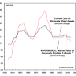
Figure 6: The World According to the Scriptures
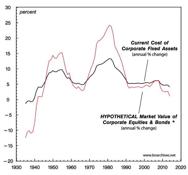
* Computed annually by adding to the historical average of the growth rate of current corporate fixed assets 2.5 times the deviation of the annual growth rate from its historical average.
NOTE: Series are smoothed as 10-year trailing averages. The last data points are for 2013.
SOURCE: U.S. Bureau of Economic Analysis through Global Insight (series codes: FAPNREZ for current cost of corporate fixed assets).
This pattern of irrationality is illustrated in Figure 6. The thick line in the chart measures the actual rate of change of fixed assets priced at replacement cost and smoothed as a 10-year trailing average.[11] Unlike the thick line, the thin line is hypothetical. It simulates what the ups and downs of capitalization might look like if investors were excessively optimistic on the upswing and excessively pessimistic on the downswing (the exact computation of the series is explained in the footnotes to the chart).
Such simulations help market analysts tease order from the chaos. They show that investors’ irrationality – however embarrassing, regrettable and inconvenient – is bounded and therefore manageable and predictable. The build-up of excessive investors’ optimism during the boom is reversed during a bust, when these very investors become excessively pessimistic. The boom-driven euphoria that gives rise to a bubble of “fake wealth” and a soaring Tobin’s Q is eventually replaced by fear, causing wealth to appear smaller than it really is and Tobin’s Q to crash-land.
7. A house of cards
So now everything finally falls into place. (1) “Real capital” cannot be measured and probably doesn’t have a unique quantity to begin with, but that’s OK if we can pretend that its magnitude is proportionate to the current price of fixed assets. (2) Tobin’s Q averages more than 1 – but that’s OK too, since the larger value can be attributed to the existence of highly productive intangible assets that, unfortunately, nobody can really see. And (3) Tobin’s Q fluctuates heavily – admittedly because the asset market is imperfect and humans are not always rational – but that, too, is fine, since the asset market’s oscillations are safely bounded, pretty predicable and, most importantly, move broadly together with “real” accumulation.
Or do they?
Notice that the capitalization series in Figure 6 is entirely imaginary. As it stands, it reflects not the reality of the market, but the assumptions of the theory – and in particular, the assumption that the growth rate of capitalization amplifies yet moves together with that of real capital. But is this a correct assumption to make?
According to Figure 7, the answer is a resounding no.
The thick line here is the same as in Figure 6. It measures the rate of change of the replacement cost of fixed assets. The thin line, though, is no longer hypothetical: it measures the actual rate of change of the value of corporate stocks and bonds. And it is here that the real/nominal duality and its associated mismatch thesis run into a brick wall. Unlike in Figure 6, where the ups and downs of the capitalization series amplify those of fixed assets, here they seem to move in exactly the opposite direction.
Note that these are not short-term fluctuations. The history of the process shows a very long-term wave pattern, with a cyclical peak-to-peak duration of 15-40 years. Furthermore the countercyclical movement of the two series seems highly systematic.
Now, unlike our previous findings in the paper, which we have agreed to overlook for argument’s sake, the inverse pattern evident in Figure 7 is patently inconsistent with the fundamental duality of real and financial capital. We can perhaps concede that real capital does not have a material quantum, and then pretend that this quantum is proportionate to the market price of the underlying capital goods. We can perhaps accept that there are invisible assets that nobody can observe, yet believe that the know-all asset market can indirectly measure them for us, as a residual. And we can perhaps allow economic agents to be irrational, and then assume that their imperfect asset pricing is nonetheless bounded, oscillating around the “true” price of real capital. But it taxes credulity to observe that the accumulation of real and financial assets move in opposite directions, yet maintain that the latter movement derives from and reflects the former.
Figure 7: U.S. Capital Accumulation: Fiction vs. Reality
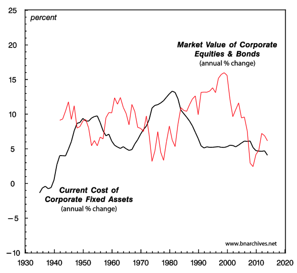
NOTE: The market value of equities and bonds is net of foreign holdings by U.S. residents. Series are shown as 10-year trailing averages. The last data points are 2014 for the market value of corporate equities and bonds and 2013 for the current cost of corporate fixed assets.
SOURCE: See Figure 4.
Present-day capitalists – or investors, as they are now known – don’t really care about “real capital”. They are indifferent to means of production, labour and knowledge. They do not lose sleep over individual rationality and market efficiency. And they can live with both “free markets” and “government intervention”. The only thing they do care about is their financial capitalization. This is their “Moses and the prophets”. The rest is just means to an end.
The promise of classical political economy, and later of economics, was to explain and justify the rule of capital: to show how capitalists, while pursuing their own pecuniary interests, propel the rest of society forward. The accumulation of capital values, the economists explained, goes hand in hand with the amassment of “real” means of production, and therefore with the growth of production, employment, knowledge, rationality, efficiency and laissez faire. But, then, if the U.S. case is representative and the growth rates of capitalization and “real capital” move not together but inversely, the interests of the capitalist rulers are pitted against those of society. And if that is indeed the case, what’s the use of economics?
8. Endgame
When capital first emerged in the European burgs of the late Middle Ages, it seemed like a highly promising startup: it counteracted the stagnation and violence of the ancien régime with the promise of dynamism, enlightenment and prosperity, and it replaced the theological sorcery of the church with an open, transparent and easy-to-understand logic. But once capital took over the commanding heights of society, this stark difference began to blur. The inner workings of capital became increasingly opaque: its ups and downs appeared difficult to decipher, its crises seemed mysterious, menacing and hard to manage, and its very nature and definition grew more slippery and harder to grasp.
Political economy – the first science of society – attempted to articulate the new order of capital. In this sense, it was the science of capital. The rule of capital emerged and consolidated together with modern science, and the methods of political economy developed hand in hand with those of physics, chemistry, mathematics and statistics. During the seventeenth century, the scientific revolution, along with the processes of urbanization, the shifting of production from agriculture to manufacturing and the development of new technologies, gave rise to a mechanical worldview, a novel secular cosmology whose intellectual architects promoted as the harbinger of freedom and progress. And it was this new mechanical cosmology – itself partly the outgrowth of capitalism – that political economists were trying to fit capital into.
Their attempts to marry the logic of accumulation with the mechanized laws of the cosmos are imprinted all over classical political economy and the social sciences it later gave birth to, and they are particularly evident in the various theories of capital. Quantitative reasoning and compact equations, Newtonian calculus and forces, the conservation of matter and energy, the imposition of probability and statistics on uncertainty – these and similar methods have all been incorporated, metaphorically or directly, into the study of capitalism and accumulation.
But as we have seen in this paper, over the past century the marriage has fallen apart. The modern disciplines of economics and finance overflow with highly complex models, complete with the most up-to-date statistical methods, computer software and loads of data – yet their ability to explain, let alone justify, the world of capital is now limited at best. Their basic categories are often logically unsound and empirically unworkable, and even after being massively patched up with ad hoc assumptions and circular inversions, they still manage to generate huge “residuals” and unobservable “measures of ignorance”.
In this sense, humanity today finds itself in a situation not unlike the one prevailing in sixteenth-century Europe, when feudalism was finally giving way to capitalism and the closed, geocentric world of the Church was just about to succumb to the secular, open-ended universe of science. The contemporary doctrine of capitalism, increasingly out of tune with reality, is now risking a fate similar to that of its feudal-Christian predecessor. Mounting global challenges – from overpopulation and environmental destruction, through climate change and peak energy, to the loss of autonomy and the risk of social disintegration – cannot be handled by a pseudo-science that cannot define its main categories and whose principal explanatory tool is “distortions”. You cannot build an entire social cosmology on the assumptions of individual rationality, equilibrium and perfect markets – and then blame the failures of this cosmology on irrationality, disequilibrium and imperfections. In science, these excuses and blame-shifting are tantamount to self-refutation.
What we need now are not better tools, more accurate modelling and improved data, but a different way of thinking altogether, a totally new cosmology for the post-capitalist age.
___________________________
SUGGESTED CITATION:
Shimshon Bichler and Jonathan Nitzan, “Capital accumulation: fiction and reality”, real-world economics review, issue no. 72, xx Oct 2015, pp. xx-xx, http://www.paecon.net/PAEReview/issue72/BichlerNitzan72.pdf
[1] This paper is an edited transcript of a March 2015 presentation by Jonathan Nitzan at UQAM, organized by AESE UQAM (Association des Étudiants en Sciences Économiques, http://bnarchives.yorku.ca/436/). An earlier and somewhat different version of this article was published in 2009 by Dollars & Sense (Contours of Crisis II: Fiction and Reality, April 28, http://bnarchives.yorku.ca/258/). Shimshon Bichler teaches political economy at colleges and universities in Israel. Jonathan Nitzan teaches political economy at York University in Canada. All of their publications are available for free on The Bichler & Nitzan Archives (http://bnarchives.net). Work on this paper was partly supported by the SSHRC.
[2] Not all political economists see themselves as either liberal or Marxist, but even the nonaligned tend to accept the fundamental division between real capital and financial assets.
[3] A subtle distinction: most Marxists accept the real/nominal duality and the difference between real and financial (or fictitious) capital. But only classical Marxists anchor their acceptance in Marx’s labour theory of value. Neo-Marxists tend to eschew value theory altogether – and, in doing so, eliminate the theoretical basis on which their notions of real and financial capital might otherwise stand.
[4] In his UQAM presentation of this paper, Nitzan asked the audience how many had heard of the Cambridge Controversy. Out of about 50 people, consisting mostly of economics students, only one raised his hand. He had heard about it in a sociology class.
[5] Apparently unbeknown to the Cambridge controversialists, this argument was articulated already at the turn of twentieth century by the American political economist Thorstein Veblen.
[6] Hard-core neoclassicists might object to this description, saying that utils are unique to the individual and therefore impossible to add across individuals to start with. However, since following this objection to the letter would make comparison and aggregation – and therefore practical economics – impossible, most neoclassical economists tend to ignore it. To bypass their own liberal-individualistic logic, they assume that all individuals are the same, that they are therefore perfectly comparable, and that their utilities can be aggregated after all. . . .
[7] The Marxist inversion would be the same, only that, instead of utils, it would generate SNALT.
[8] Neoclassical economists insist on distinguishing between average and marginal utility. But since utils are forever invisible, and given that, in the interest of aggregation, neoclassical individuals are reduced to identical drones with homothetic preferences anyhow, this distinction need not distract us.
[9] For more on the classical Marxist treatment of capital, see Chapters 6-8 in our book Capital as Power: A Study of Order and Creorder (Routledge, 2009, http://bnarchives.yorku.ca/259/). It is important to mention here that, in their empirical research, most Marxists have thrown in the methodological towel. Instead of relying on labour time and the dialectical method, they use “real” neoclassical data, liberal classifications and equilibrium-based econometrics. This wholesale surrender is akin to physicists reverting back to astrology and chemists back to alchemy. Moreover, most Marxists rarely acknowledge, let alone assess, the implications of this surrender – and the handful who do often end up defending it!
[10] A note to the uninitiated: the term “economics” was coined at the end of the nineteenth century by Alfred Marshall, who thought that “political economy” was insufficiently scientific, and that a suffix of “ics” would make it sound much more respectable, like mathematics and physics.
[11] Note that this series excludes intangibles, but since we are displaying here not levels but rates of change, we can conveniently assume that the sum of tangible and intangible assets would follow a growth pattern similar to that of the tangible assets only.
Donating = Changing Economics. And Changing the World.
Evonomics is free, it’s a labor of love, and it's an expense. We spend hundreds of hours and lots of dollars each month creating, curating, and promoting content that drives the next evolution of economics. If you're like us — if you think there’s a key leverage point here for making the world a better place — please consider donating. We’ll use your donation to deliver even more game-changing content, and to spread the word about that content to influential thinkers far and wide.
MONTHLY DONATION
$3 / month
$7 / month
$10 / month
$25 / month
You can also become a one-time patron with a single donation in any amount.
If you liked this article, you'll also like these other Evonomics articles...
BE INVOLVED
We welcome you to take part in the next evolution of economics. Sign up now to be kept in the loop!
